
Background
The project centers on how to enhance the audio signals through a microphone array. So the algorithm includes beamforming, sound source localization. Mathwork offers us the Phased Array System Toolbox today, we can directly finish the program of microphone array quickly, here it is my personal project and optimizes part of the code in frequency domain from time domain.
Technical Objective
The main program consists of the beamforming, localization of a sound source. For the beamforming, I implement delay-and-sum, and robust GSLC. For the sound location, I implement SRP PHAT. (The original code reference from The University of Kentucky)
Beamforming
The sensitivity pattern is similar to a beam, people define it beamforming. By using multiple microphones to combine the signals, so as to listen in the desired direction of the sound source, and have effect on suppression of the noise, echo, reverberation from space elsewhere.
There are two major groups of microphone-array algorithms: time-invariant and adaptive. Here are delay-and-sum Beamforming and GSCL Beamforming behind. It should be noted that the location of a sound source is known when talking about beamforming then I will show how to localize a sound source with SRP PHAT.
1.Delay-and-Sum Beamforming
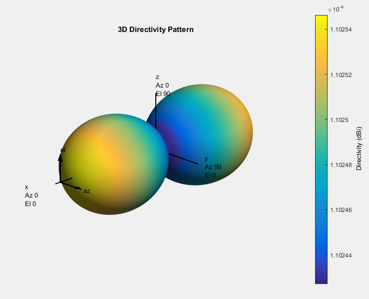
For this kind of beamforming, I think it is better in time domain than in frequency domain, because its delay is easily applied in real time through time domain. Assuming the location of a sound source in Cavendish coordinates and ideal omnidirectional microphones, I check the main lobe of the microphone array by Pattern and Phased command. Because of the rectangular array, I choose Phased.URA and Pattern. The code below.
h_rec = phased.URA(‘Size’,[2 2],’Lattice’,’Rectangular’,’ElementSpacing’,[1,1]);
c = 340;
freq = [300 1e4];
plotFreq=linspace(min(freq),max(freq),5);
figure
pattern(h_rec,plotFreq,[-180:180],0,’CoordinateSystem’,’rectangular’,…
‘PlotStyle’,’waterfall’,’Type’,’powerdb’,’PropagationSpeed’,c)
figure
Freq=5e3
pattern(h_rec,Freq)
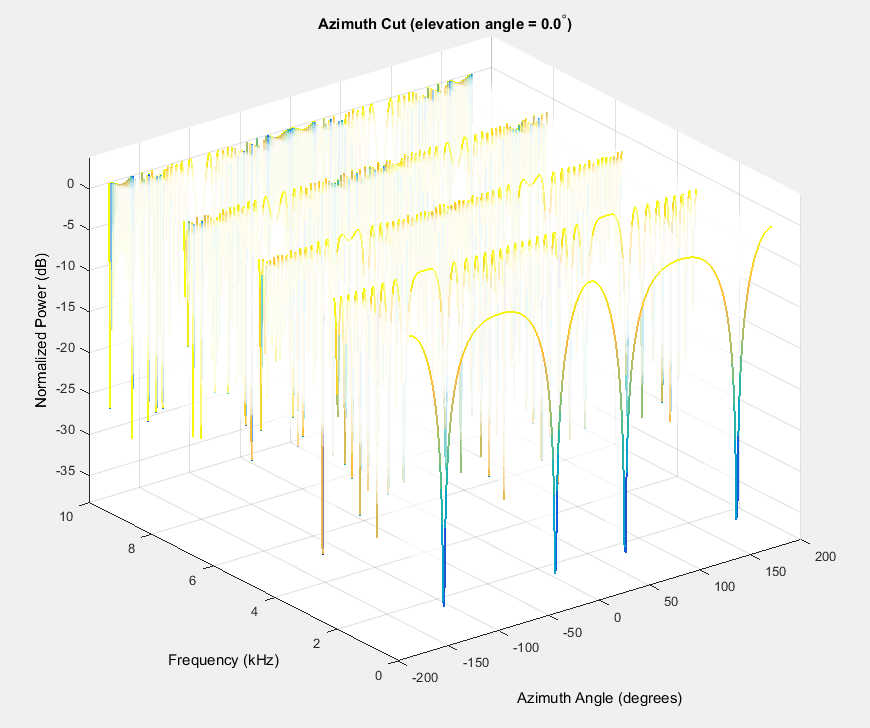
The delay beamforming effect can delay the several signals in different channels to align signals reaching the microphone at the different time, and by summarizing the multiple signals after the delay. The noise will subtract each other due to the different phase. That is a delay-and-sum Beamforming, as shown in Figure . For signals, there are two options to dispose of the signals, advanced or delayed, when samples are stored in memory. The code of delay-and-sum
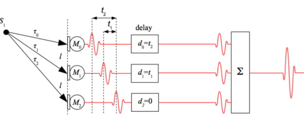
Figure Delay-and-sum
2. Robust GSCL Beamforming
Adaptive processing algorithm performs better to estimate the weights in real time and achieve better noise suppression, according to the microphone-array geometry and the input signals, but it costs more memory and CPU power.
Objective of robust GSCL beamforming
GSCL Beamforming is efficient to reduce the interference with a number of microphones. It achieves the signal from the direction of arrival. However, it is confined when the nulls are sharp and the desired signal is removed by the blocking matrix. So Hoshuyama designed the robust to address the issue, (reference from Hoshuyama). The scheme of the robust GSCL Beamforming shows in Figure 3
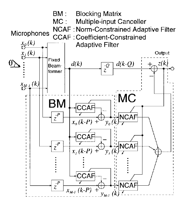
Figure Architecture of robust GSCL Beamforming
The design of robust GSCL beamforming
the robust GSCL beamforming consists of blocking matrix and multiple-input canceller. It contains norm-constrained adaptive-filter (CCAF) and coefficient-constrained adaptive filter (NCAF), on another view angle, it is similar to a sequence combine of two adaptive filters.
The purpose of CCAF is to cancel the undesirable influence of steering-vector errors, and NCAF prevents the target-signal cancellation.
Prior to understanding the robust GSCL beamforming, it’d better figure out adaptive filter. In a word, the adaptive filter maximise the signal-to-noise raito by minimizing the total power at output of canceller. There is video online about adaptive filter
The signal relationship in the blocking matrix with N-tap CCAF is
\({ y }_{ m }\left( k \right) ={ x }_{ m }\left( k-P \right) -{ H }_{ m }^{ T }\left( k \right) D\left( k \right)\)
where
\({ H }_{ m }\left( k \right) \overset { \triangle }{ = } { \left[ { h }_{ m,0 }\left( k \right) ,{ h }_{ m,1 }\left( k \right) ,…,{ h }_{ m,N-1 }\left( k \right) \right] }^{ T } \)
\(D\left( k \right) \overset { \triangle }{ = } { \left[ d\left( k \right) ,d\left( k-1 \right) ,…,d\left( k-+N+1 \right) \right] }^{ T }\)
\({ y }_{ m }\left( k \right) \) is mth output
\({ x }_{ m }\left( k \right) \) is mth microphone signal
P is the delay number
\({ H }_{ m }\left( k \right) \) is the coefficient vector of the mth CCAF
Using the normal-least-mean-squares to adapt the coefficient
\({ h }_{ m,n }^{ ‘ }={ h }_{ m,n }\left( k \right) +\alpha \frac { { y }_{ m }\left( k \right) }{ { \left\| D\left( K \right) \right\| }^{ 2 } } d\left( k-n \right) \)
\({ h }_{ m,n }\left( k+1 \right) ={ \phi }_{ m,n }\quad \) for \({ h }_{ m,n }^{ \prime }>{ \phi }_{ m,n }\quad \)
\({ h }_{ m,n }\left( k+1 \right) ={ \psi }_{ m,n }\) for \({ h }_{ m,n }^{ \prime }<{ \psi }_{ m,n }\quad \)
\({ h }_{ m,n }\left( k+1 \right) ={ h }_{ m,n }^{ \prime }\) otherwise
(m=0,1,…,M-1), (n=0,1,…,N-1)
\({ \phi }_{ m,n }\) is upper limits
\({ \psi }_{ m,n }\) is lower limits
The signal relationship in the mulitple-input canceller matrix with N-tap NCAF is
\(z\left( k \right) =d\left( k-P \right) -\sum _{ m=0 }^{ M-1 }{ { W }_{ m }^{ T }\left( k \right) } { Y }_{ m }(k)\)
where
\({ W }_{ m }\left( k \right) \overset { \triangle }{ = } { \left[ { w }_{ m,0 }\left( k \right) ,w_{ m,1 }\left( k \right) ,…,w_{ m,N-1 }\left( k \right) \right] }^{ T }\)
\({ Y }_{ m }\left( k \right) \overset { \triangle }{ = } { \left[ { y }_{ m,0 }\left( k \right) ,y_{ m,1 }\left( k \right) -1,…,y_{ m,N-1 }\left( k-L+1 \right) \right] }^{ T }\)
Coefficients of the NCAF’s are updated by an adaptive algorithm with a norm constraint
\({ W }_{ m,n }^{ ‘ }={ W }_{ m,n }\left( k \right) +\beta \frac { z\left( k \right) }{ { \sum _{ j=0 }^{ M-1 }{ { \left\| { Y }_{ j }(k) \right\| }^{ 2 } } } } { Y }_{ m }\left( k \right) \)
\(\Omega =\sum _{ m=0 }^{ M-1 }{ { \left\| { W }_{ m }^{ ‘ } \right\| }^{ 2 } } \)
\({ W }_{ m }(K+1)=\sqrt { \frac { K }{ \Omega } } { W }_{ m }^{ ‘ }\) for \(\Omega >K\)
\({ W }_{ m }(K+1)={ W }_{ m }^{ ‘ }\) otherwise
(m=0,1,…M-1)
\(\beta \) step size
\(\Omega\) total squared-norm of \({ W }_{ m }\left( k \right) \)
K is threshold
MEX file Conclusion
I transform the GSCL code into a MEX file in floating point, it will be the fixed-point number in frequency domain in the future.(reference from the University of Kentucky) .
SRP PHAT sound location
As my assumption of knowing the location of a sound source, from now on, using algorithms to detect the localization and tracking of it. Generally, there are two distinct approaches to estimate the direction, based on time-delay estimate and based on the steered response. Here is SRP PHAT to sound location estimation.
The steered-response power (SRP) of methods forms a conventional beam, scan it over the appropriate region of the working space, and plots the magnitude squared of the output. The peak of power in the map is the sound source. The conventional beam can be a delay-and-sum beamforming. The power at the beamforming output is
\({ P }_{ bf }(c)={ D(c) }^{ H }SD\left( c \right) \)
Here, S is the cross-power matrix of the input sample, \(S\overset { \triangle }{ = } X{ X }^{ H }\). and \({ D }_{ c }(f)\)
The PHAT weighting is
\({ P }_{ SSL }\left( c \right) =\frac { 1 }{ K } \sum _{ k=1 }^{ K }{ \frac { M }{ { X }_{ k }^{ H }{ X }_{ k } } } { P }_{ SSL }\left( c,k \right)\)
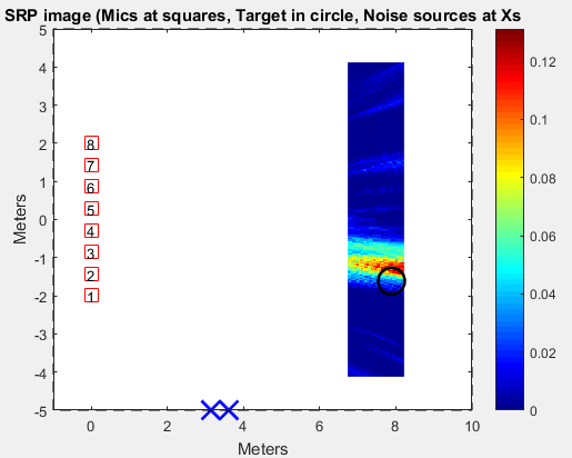
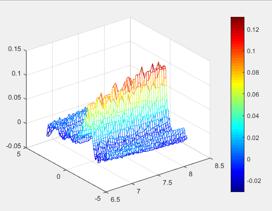
If setup eight microphones in a line, two noise in a wall, I can have the SRP image whose red color peak is where the sound localizes. The SLL code. (The reference from The University of Kentucky)
Conclusion
Today people can directly finish it through Matlab Toolbox, instead of all above. According to its report in Matlab, if the microphone array is the rectangular with four microphones, its delay-sum beamforming can increase 4.5915 dB, and Frost beamforming can increase 7.4682 dB.