
Background
Thermal management is a significant challenge in advanced aircraft, rocket, and missile engines. As flight speeds increase to the high supersonic and hypersonic level, the temperature of the air taken on board becomes too high to cool the structure and, therefore, it is necessary to use the fuel as the primary coolant.
Aerojet Rocketdyne in cooperation with the Florida Institute of Technology (FIT) to improve their state of the art hypersonic propulsion thermal ‘model’ and material capability.
I worked with Adrien Jasinski. Our task was the installation of all the electrical components for the experiment and the development of a program to control and setup the experimentation
Technical Objective
a. General purpose
The main goal of this collaboration between Aerojet Rocketdyne and FIT is to improve Aerojet Rocketdyne’s modeling capability and reduce predictive uncertainty in a flight-like hydrocarbon fuel-cooled heat exchanger.
Adrien Jasinski and I worked on the first phase of the Hypersonic Propulsion Heat Transfer by exploring coolant side convection in a flight-like configuration. The second phase will concentrate on hot side heat transfer.
A functional diagram of the experiment is shown in Figure 1 (Process and control diagram). The aim of this experiment is to simulate the heat exchange conditions that can be found in a propulsion system for aircraft, rockets or missiles.
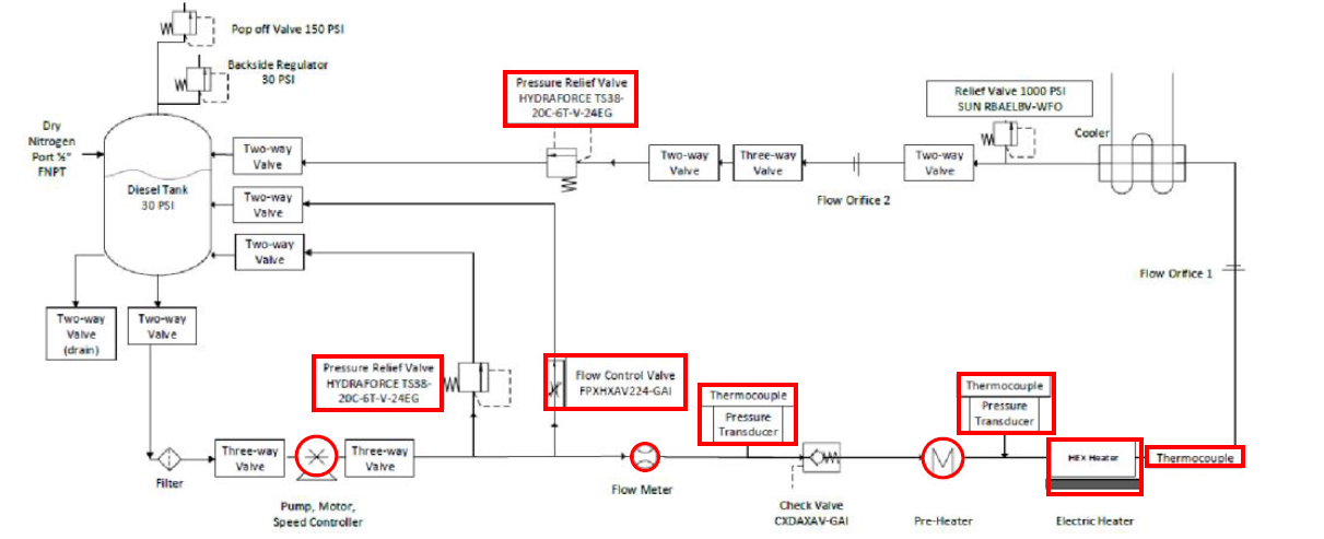
Figure 1 Process and control diagram
The rig includes an electrical pre-heater, a main electrical heater, and a flow rate control, to be used to create the desired inflow conditions, with inflow temperatures up to 1000 F.
Diesel is used for testing the proper function of the experiment minimizing risk. In the future, it will be possible to use other exotic gases. The red components in the diagram, ( Figure 1) are installed and they are all connected to a computer for data acquisition and control.
The data collected from this experiment include the fluid inlet and outlet temperature from the heat exchanger for a given flow rate. After the acquisition, this data will be compared with well-established heat exchanger performance to confirm the proper performance of the experiment.
Thermal development length and variation as the coolant heats up are quantified by thermocouples located along the length of the heat exchanger. Other thermocouples are placed before and after the heat exchanger to measure the performance of the heat exchanger. Figure 2 presents a surrogate of the heat exchanger; the real heat exchanger is kept secret by Aerojet Rocketdyne and the FIT.
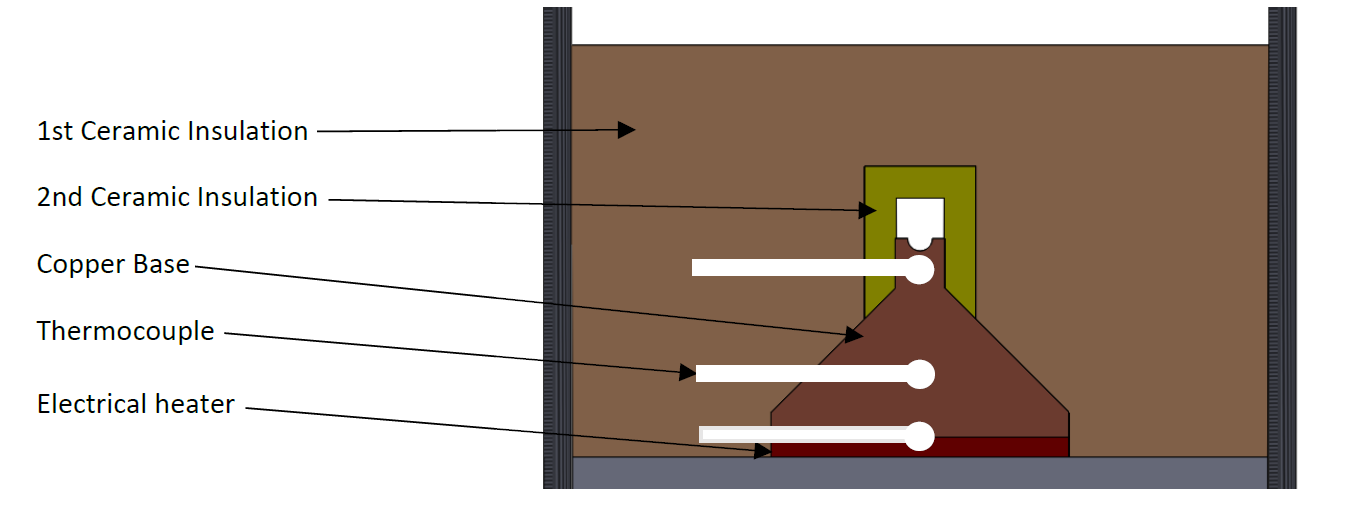
Figure 2 Schematic surrogate of the heat exchanger
The rig uses a high-pressure nitrogen tank to pressurize the dump tank (30 psi). The surrogate heat exchanger is heated by an electrical heater which can provide heat to the fluid to cover all the required operational conditions with a sufficient margin. A pre-heater enables the fluid to be at 1000 F inflow. The surrogate heat exchanger is heated on a copper base to provide uniform heat transfer. The flow of diesel in the pipe is controlled with a pump motor by reducing or increasing the speed of the motor.
b. Hardware and environment
From this diagram Figure 1, the goal was to install all the sensors (thermocouples, pressures sensors, flow meter) and devices (pump, heaters, valves) and to control every device from a computer with the software LabView. All the devices were already bought but not installed.
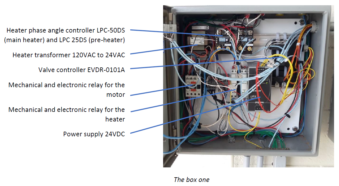
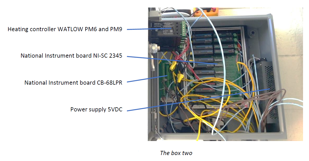
We fixed two national instrument boards (LabView controller) in a box (figure 3). These boards are able to control the motor of the pump, three electrical valves and they can collect the temperature of six thermocouples and three pressure sensors. The two boards are directly connected with the computer with a dedicated National Instrument cable.
Two heating controllers (the two black devices in front of the box 2 figure 3) and the computer are connected with a USB RS485.
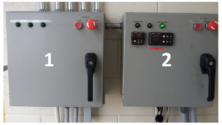
Figure 3 Close boxes with electrical controls
It is important to control all the experiment from a computer for safety reasons, a lot of walls separated the operator from the high pressure and high temperature (figure 4). Again, for safety reasons different emergency buttons were installed on the boxes to cut the current to the pre-heater, main heater and the motor in case the computer couldn’t send the command to the electronic relay.
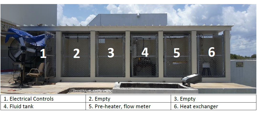
Figure 4 The site of the experiment
The fourth compartment was equipped with the pump-motor, the tank (figure 5)with a pressure sensor on it and three electrical valves. On these three electrical valves, only one was used that time: a pressure valve. The two others could be used in order to change the way of controlling the flow rate of the liquid, indeed this time these valves were open and the flow rate was controlled by a pump.
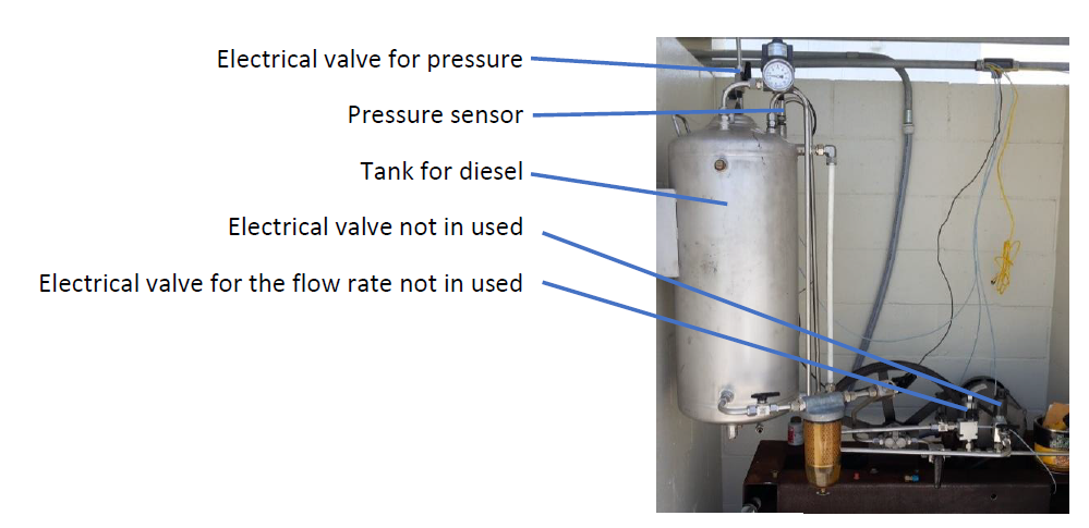
Figure 5 Tanks and valves
Figure 6 shows you the fifth compartment of the experiment. In this compartment, we were reading the flow rate with the flow meter (in red), the temperature (thermocouple in yellow) and the pressure before the fluid goes into the heat exchanger. The pre-heater is a heating cord wrapped around the tube.
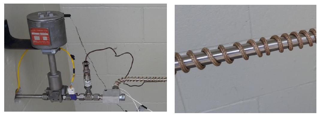
Figure 6 Flow meter and pre-heater
Figure 7 shows the last compartment of the experiment. It is composed of the main heater, the surrogate of the heat exchanger and three thermocouples. The three thermocouples are installed on the surrogate heat exchanger at different positions: one in contact with the main heater, one in contact with the pipe and one between the two others. These three thermocouples will give us information about the variation of the heat exchanger. The last thermocouple is installed at the outlet of the heat exchanger, it will give us the performance of the surrogate heat exchanger by comparing the inlet and outlet temperature of the heat exchanger.
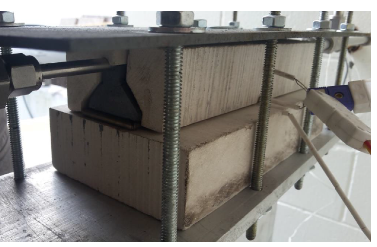
Figure 7 Surrogate of the heat exchanger
c. Software
LABVIEW
We had to acquire and visualize data sets rapidly from different Input and Output devices so we used LabView to simplify hardware integration and data acquisition. Indeed this software has a good interface for acquisition of data and instrument controls: there is a graphical interface for programming (using block diagram) that allows us to reduce programming time and a front panel was used at the end of the programming to start the acquisition, visualize data and control the instruments (figure 8).
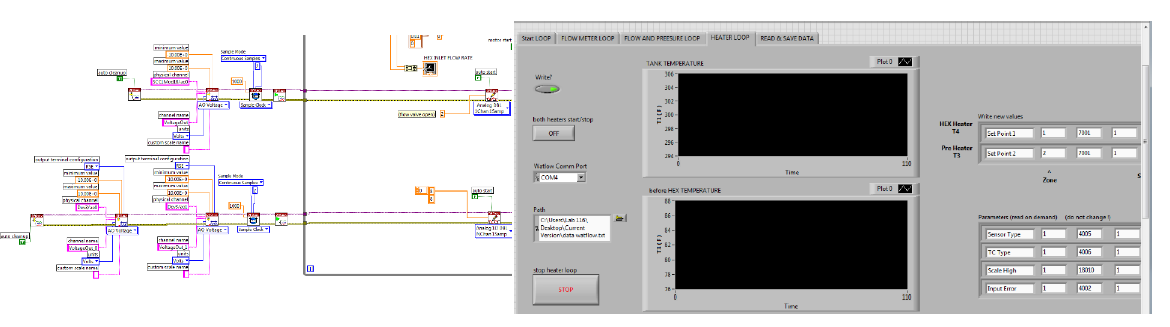
Figure 8 Graphical interface and front panel on Labview
WATLOW EZ-ZONE
To regulate the temperature of the two heaters, the LabView program sends the set point chosen by an RS485 communication port to two Watlow heating controllers. These Watlow controllers also receive the temperature from two thermocouples and they are able to regulate the temperature on their own thanks to a PID loop included in the device. The output of the device is a tension from 0V to 10V sent to two heater angle phases. These two heater angle phases adjust the high tension 120V to the heaters proportionally to 0-10V from the WATLOW controllers. The main problem we had with these Watlow controllers was the setting of every parameter of the PID. Indeed, without setting properly these parameters the two heating controllers would not regulate the temperature correctly.
Figure 9 presents the parameters chosen for the PID of the two WATLOW controllers.
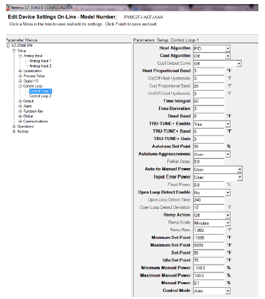
Figure 9 Watlow EZ-Zone Software
We played on three different parameters: Heat Proportional Band, Time Integral and Time Derivative. All the values chosen in the PID parameters were set without fluid in the pipe. Other values could be set when the experiment will run with the diesel.
Heat Proportional Band sets the gain for PID control. Larger proportional band values correspond to less gain. After some tests with our system, we determined that it was better to set a low value on this parameter.
Time Integral sets how aggressively the integral part of the PID algorithm acts. Integral acts to drive the process value to set point by steadily adjusting the output whenever the process value deviates from the setpoint. A shorter Time Integral setting yields a larger power adjustment for a given deviation from a set point over a given time. In our case, it was better to have a high value on this parameter.
Time Derivative sets how aggressively the derivative part of the PID algorithm acts. Derivative acts to prevent the process value from changing too quickly. Too much derivative can slow the process to adjust to changes. A longer Time Derivative setting yields a greater power adjustment for a given change. In our case, it was better to have a low value on this parameter.
Changing the tuning values during the process may also improve the control. For that, we set TRU-TUNE+ to on to adaptively tune the value of the PID while the process was running.
Autotune Aggressiveness selects the responsiveness of the auto-tuning process. In our case it was better to use “over”, it will respond slowlier but will avoid or reduce overshoot.
Programming
The final program on LabVIEW works with five different sequences as follow. All general schematic in Figure 10
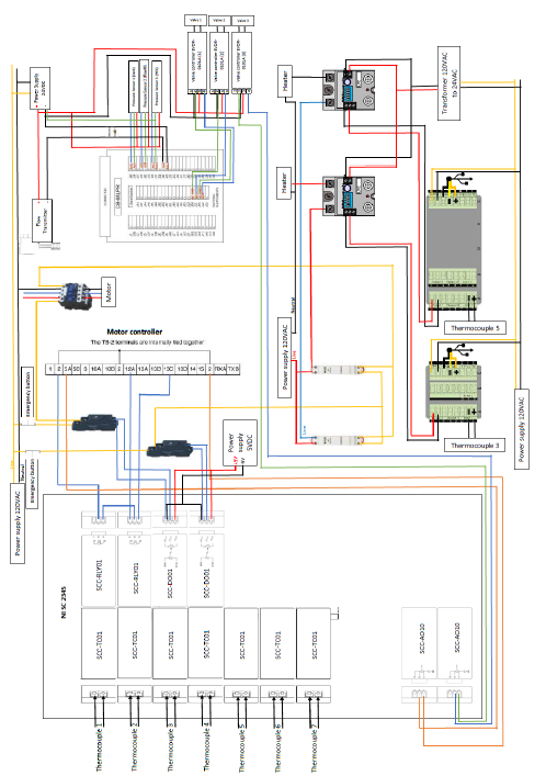
Figure 10 General Schematic of electronic components
All front panels of each sequence are available in next illustrations
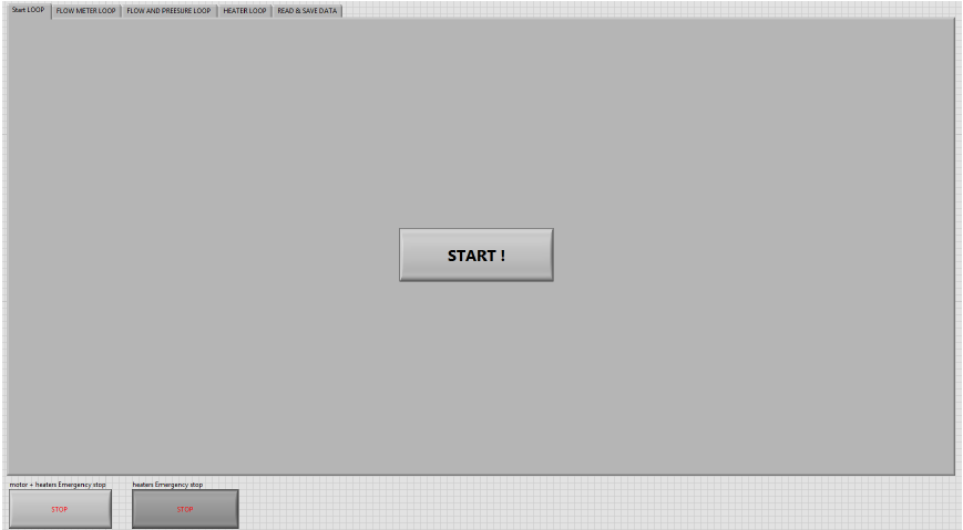
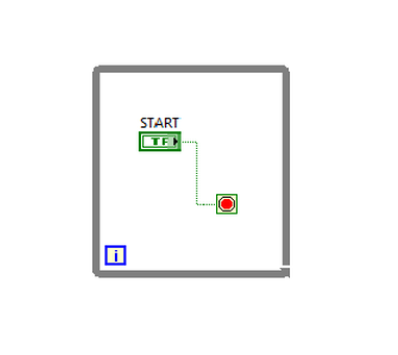
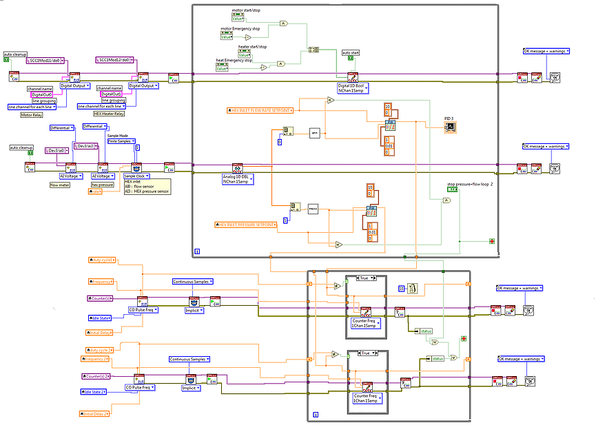
The first sequence starts the program and goes to the second sequence, it is the start loop.
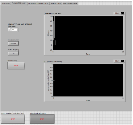
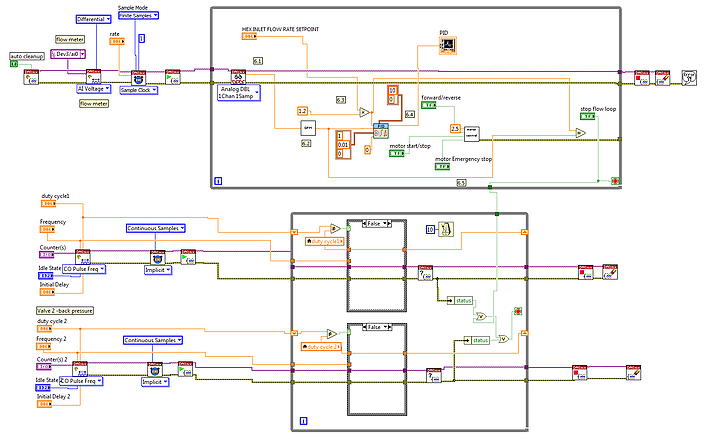
The second sequence declares different channels and allows the operator to set up the value of the flow rate into the heat exchanger inlet, it is the flow meter loop. Channels declare are:
- One digital output to engage the motor
- One analog output to regulate the speed of the motor
- One analog input to take the measure from the flow meter
- Three analog outputs to open or close two proportional valves and one flow valve
On this sequence there is a control loop feedback mechanism : we used a PID controller function to calculate continuously the differences between the desired set point (the mass flow) and a measured process variable (the flow rate from the flow meter) and applies a correction based on proportional, integral, and derivative terms on the speed of the motor. On this sequence the PID value of the different valves were set as default, there was no feedback control on it.
The third sequence allows the operator to choose the pressure in the heat exchanger inlet, it is the flow and pressure loop. As the flow rate in the second sequence, the pressure is regulated with a PID controller function: the set point is the pressure, a measured process variable is given by a pressure sensor and the difference between the two values will be processed by the PID and a correction will be applied thanks to a pressure valve to regulate the pressure. In this sequence the flow rate remains the same as in the previous sequence.
The fourth sequence allows the operator to choose the temperature of the pre-heater and the main heater, it is the heater loop. The temperature is regulated differently than the flow rate and the pressure in the previous sequences. Indeed, as I was explaining in II.2.b. and c., heaters are controlled with two heating controllers Watlow PM9 and PM6 and these devices have their own control loop feedbacks. In the program, set point values chosen by the operator are sent to the heating controllers by RS485 and thanks to a thermocouple connected to the Watlow devices the temperature is regulated by an intern PID.
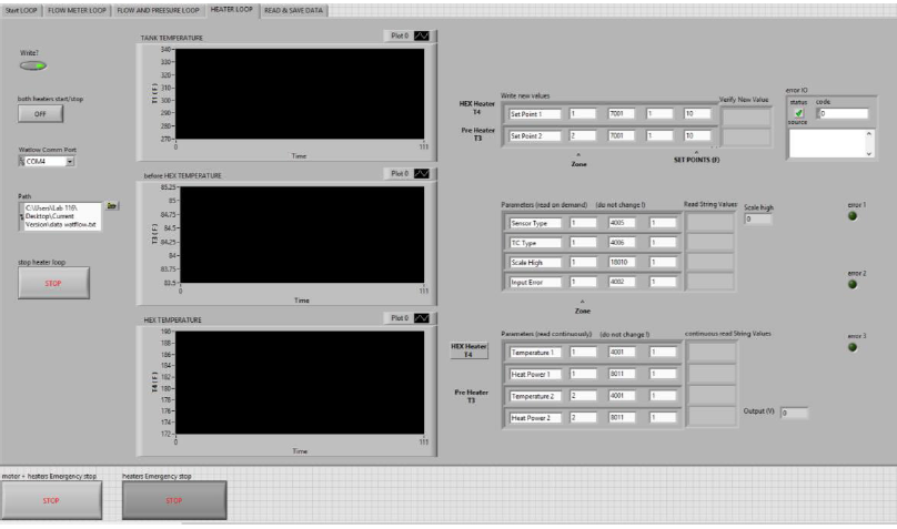
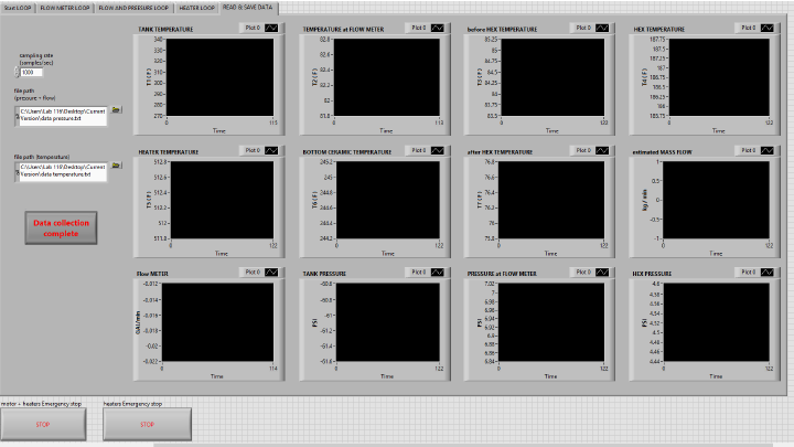
The fifth and last sequence allows the operator to read the measurement of every sensors to ensure the proper functioning of the experiment and to check that the temperature, the pressure and the mass flow chosen achieve the right value, it is the read and save data loop. When the values are reached, all the data of every sensor can be collected by clicking on data collection complete and all the data will be saved in a file in .txt. Then the program ends by clicking on stop motor + heaters.functioning of the experiment and to check that the temperature, the pressure and the mass flow chosen achieve the right value, it is the read and save data loop. When the values are reached, all the data of every sensor can be collected by clicking on data collection complete and all the data will be saved in a file in .txt. Then the program ends by clicking on stop motor + heaters.
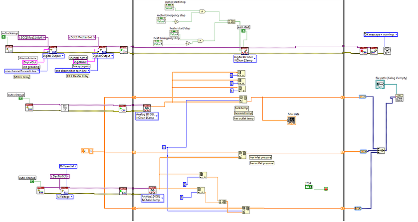
In addition to physicals emergency buttons to cut the current it is also possible to stop the motor and the heater on every sequence of the program. This is made possible thanks to electronic relays adapted to National Instrument boards.
Conclusion
I do not finish the data collection because the flow measure was broken, but after it is fixed, it worked right. The data from the experiment will be used to develop a new engine.